Basic Iterative Numeric Optimization
Today in a class, we were asked to write an iterative solver for numerical equations. Now, many students in the class did not have an optimization background, so for the benefit of everyone, I want to share a simple overview of this exercise and how to go about solving it.
The problem was stated as follows:
$$ M(a) = 2\times a + 14 $$ $$ G(b) = b - 2 $$
And our goal was to find some solution $x$ such that $M(x) = G(x)$. Additionally, we were supposed to do so iteratively, so just solving the system of equations was out of the question. This is because our next exercise would have a different $M$ and $G$, so our code should be able to support whatever.
For the sake of generalization, my solution here will assume only the $M$ and $G$ are continuous, but I will not assume we know their derivatives. Additionally, I will be writing my code in python, simply because I find that it is easier for anybody to understand. Knowledge of python, hopefully, won’t be necessary. But first, lets go over some aspects of the problem…
What is an iterative algorithm?
As stated above, we are going to write an iterative solution, which means that our code will start with a random guess and refine it over time.
Why write an iterative algorithm?
In the real world, we won’t know everything about $M$ and $G$. They may be uncertain, ill-defined, or the result of a large simulation. So we wouldn’t be able to simply solve a system of linear equations. By using an iterative method, we can treat each function as a black box. This just means that our code won’t know what $M$ or $G$ actually do, but it will be able to evaluate each function at different points.
How do we write an iterative algorithm?
First, we are going to make a random guess at $x$. Then, we are going to check if our guess is right. If our guess is wrong, we are going to check whether we need to increase or decrease $x$ to get closer to the right answer.
Caveat: Every optimization algorithm is going to answer the question, “How do I update $x$?” a different way. The method presented here is very simple, for the same of explaining the overarching concept.
Conceptual Solution
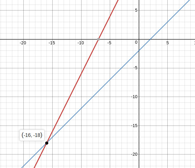
For future reference, here are our two functions shown graphically. Note that to make these plots we need to know the values of $M$ and $G$ at EVERY $x$ value. In real life this is impossible, so instead we are going to do this iterativly. But, this sort of check, for a simple problem, is a good idea just to know what the right answer will look like, regardless of method. In this case, our solution is $x = -16$.
Lets start our iterative process with a random guess, $x = 1$. We know we want $M(x) = G(x)$, but we can simplify our analysis by defining a third function: $D(x) = M(x) - G(x)$. Clearly, if $D(x) = 0$, we have our answer.
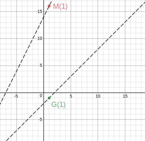
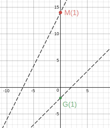
At this point, all we know is that $M(1) = 16$ and $G(1) = -1$, so $D(1) = 17$. Graphically, this is just the two points shown below (dashed lines for reference, we don’t know those yet).
So, we need to figure out whether we need to increase or decrease $x$ to get closer to a solution. For this, we are going to estimate the derivative of $D$. To do this, we just evaluate $D(x)$ at two points close to our previous guess. For example:
$$ D(1.01) = 17.01$$ $$ D(.99) = 16.99$$
We use this to estimate the derivative of $D(1)$, which is simply change in y over change in x:
$D’(1) \approx 0.02 / 0.02 = 1$
So our best guess, is that if we decrease x by 1, our difference will also decrease by 1. Note that this only requires we evaluate $D(x)$ at two points, and we don’t need to know the entire function to make this derivative estimate. So for our next iteration, let $x=0$.
Sure enough, $D$ decreased by 1. If we were to follow the whole algorithm threw, we would make another derivative estimate and eventually find our solution of $D(16) = 0$.
Considerations
A couple of things were hand-waved away so far. Firstly, how far away from $x$ do we need to look in order to calculate the derivative? Also, how far should we jump once we have a local derivative estimate? Finally, what if we jump past the right answer?
In this example, we only have linear equations, so as long as we take small steps, we will eventually get it right, but in the case of more complicated polynomials. In more complicated equations, we may get stuck at local optima, where no mater how we move $x$ we seem to only get further from $D(x) = 0$. That typically is solved by running our overall solution with multiple random guesses, or by varying the step size. But, lets get this solution programmed first.
Code
from random import random
# If you don't know python, don't worry about this import

# function for M
def M(x):
  return 2 * x + 14

# function for G
def G(x):
  return x - 2

# function for the difference of M and G
def D(x):
  return M(x) - G(x)

# estimates the derivative of D at x.
def estDerivative(x):
  STEP = 0.01
  # sample D at two points near x
  e1 = D(x-STEP)
  e2 = D(x+STEP)
  # return rise over run
  return (e2 - e1) / (2 * STEP)

# dermines how far to move x each iteration
# also, the smaller the jump, the closer
# we end up to the right answer
JUMP = 0.0001

# start with a random guess for x
x = random()

# keep looping until the absolute difference
# between M and G is (practically) 0
while abs(D(x)) > 0.001:
  # calculate change in D for change in x
  d = estDerivative(x)
  if D(x) > 0:
    # if positive, we need to update x against the direction of d
    x += -d * JUMP
  else:  # D(x) < 0
    # if negative, we need to update x along the direction of d
    x += d * JUMP

print(x)