I’ve found it interesting how a lot of the conversation about embedding models and other neural network models haven’t really converged. Something that seems to complicate the issue is that Tensorflow as an object called “Embedding”. So the following describes some high-level understanding about how neural networks relate to other embedding methods.

So an “embedding” is a simplified vector representation of something, and I phrase it like that because embeddings happen everywhere for neural networks, not just for text. Imagine we wanted to classify small pictures of handwritten digits. Imagine our images are grey 32x32 pixel squares like this:

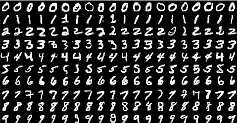
In this simpler example, we can just flatten our image into a 1024-dimensional representation, each dimension representing the “brightness” of a single pixel.

Okay so now where embeddings come into it. We know that there is an underlying 10-dimensional embedding that captures all the important information in these pictures, because we know the pictures represent the 10 digits. So we can use a neural network to learn these dimensions. Because our 10-dimensional space is much smaller than the input 1024-dimensional space, we are going to have to “throw away” a lot of information. The properties of our neural network, including the number of layers and the size of each layer, determine how “quickly” this will happen.

To understand this, first a little bit on how neural networks predict things This is the most fundamental operation in a neural network.

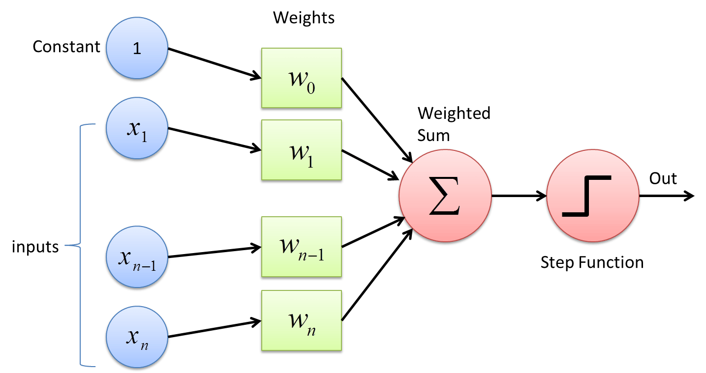
Given a vector, the network multiplies each dimension by a weight, sums the results, and runs that through an activation function. If this activation function were linear, then this would simply be a linear combination, and I find that is a strong way to intuit about this. If we have two dense layers in our neural network, the first of size $m$, the second of size $n$, then every element of the second vector is simply a different linear combination of the first.

Okay so back to recognizing handwritten digits. If our neural network contained only two layers, one for the 1024-dimensional input, and a second for the 10-dimensional output, then that would imply that each digit could be recognized through a simple linear combination of the pixel values. One notation for this network is “1024-10” This discards a lot of information about the grouping or order of the pixels, and instead the model would have to learn which individual pixels were most important to specific digits. The end result might learn something that the top-left pixel is the most important to the number 3.

To learn more complicated relationships, we can add more layers. The rule-of-thumb is that intermediate layers should be half the size of the previous layer. So, we could create a network that started with the input, then created an intermediate “embedding” of size 512, and then finally outputting the 10 digits. This would be “1024-512-10”. Now we learn 512 different linear combinations of our input. Each one might capture a different pattern of pixels that are useful. For instance, one pattern could highly weight pixels around the center, which would be common for digits like 0, 6, and 8. Then, we would learn a second linear combination to get output 10 digits. However, now we are learning a combination of combinations. For instance, the number 0 might be most likely if we have many bright pixels in the center, and no pixels around the edges.

There is very little practical formula that can tell is if that “1024-512-10” model is good enough. Maybe we want “1024-512-256-10” or more? While “deeper” models (those with more layers) can capture more complex structures, they also can “overfit”. This would mean in the example case that the model learns a specific pattern for each image its ever seen, and has no clue what to do with future information. This is where experimentation comes in. A good rule of thumb is to try and have 10 training examples for each parameter. In a neural network, each weight of each combination is a parameter. In the “1024-10” network, there are 10,240 weights. In the “1024-512-10” network there are $1024 \times 512 + 512 \times 10 = 529,408$ weights. This is why neural networks require tons of training data to work.

Okay now lets get to text embeddings. The simplest “embedding” of text is the “one-hot” representation. Imagine we were working with a set of documents that contained 5-million unique English words. A one-hot embedding would represent each word as a 5-million dimensional vector. For many practical reasons, we can’t use that. But also, treating each word uniquely has the same limitations as looking at individual pixels. So instead, we are going to use an “embedding” of words that reduces the dimensionality of words to something we can actually use. But its also going to capture some interesting patterns present within language, in the same way that we might have learned patterns in images above. However it doesn’t need to be that fancy.

In machine learning libraries like Tensorflow, they provide an “Embedding” object. All this does is perform a lookup for each one-hot vector in a very optimized way. These embedding start out randomly initialized, and during training are updated like any other layer. However, because these are typically very large objects (a 100-dimensional embedding of 5-million words would include 5 billion parameters), we often do some tricks to make them more usable. But, without a any fancy pretrained embedding, we could perform sentiment analysis like this: Step 1: lookup the embedding of each word in a document Step 2: average that result together Step 3: apply regular neural network layers to reach a desired result. However, remembering the rule that says we need 10 training samples per parameter, using this text embedding method would be infeasible for every text problem we come across.

The reason we don’t do this is because transferring embedding from a different, more generic problem, often leads to much better models. The generic problem that we pick must only be solvable if the embeddings of each word capture some useful information about each word. We can then train a model that solves this problem, and re-use those embeddings everywhere. The problem we often pick is to predict the likely neighbors of each word. This is captured by the skip-gram model.

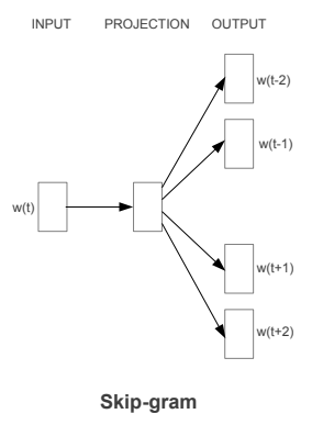
So we take our set of documents and pick out a “window” This includes a “target word” as well as “w” words before and after it. If the word “documents” was the target word of a window from the first sentence of this paragraph, a window might be: (our, set, of, and, pick, out) The skip-gram model begins by looking up an embedding of “documents” and then attempts to predict the other six words.

Google performed their news corpus of over 7-billion documents, which comprised of likely over 100-billion windows. At that scale, we will see the word “documents” occur next to thousands of relevant related keywords. More important, we will see words like “paper” or “file” appear in similar company. As a result, we start to learn some very useful patterns in language. And again, because this problem is much easier to solve than typical machine learning tasks, it was feasible for Google to scale up to a place where they are meeting that 10-example-per-parameter scale.

So when we use embeddings in a project, we are going to be taking some pretrained values for our models. This allows us to leverage the work bigger groups have already done to learn some very nontrivial patterns in language. We can then learn our own patterns-of-patterns from this data, that better fits our own applications.