Recently, in text mining circles, a new method of representing words has taken off. This has been due, in a large part, to recent papers from Mikolov et al. and tools like word2vec ¹. Since then, many other projects have applied this concept to a wide variety of areas within data mining ². So what is all the hype about? What are these embeddings and why do we need them?

What is a word embedding?

So the word “embedding” is vague, and often times the same thing will be referred to as a “representation.” These terms clearly aren’t clear. When we say we want to find “word embeddings” or “word representations” we mean that we want to find numerical representations for a set of words from a set of documents. Of course, the question is “how?” Or maybe, the question is “why?”

“Why?”

Well, text is very difficult for a computer to process. People write in very expressive ways, and the meanings of words change over time. Because of this, there are very few machine learning methods which accept “text” as input. On the other hand, practically every method accepts a vector as input.

So imagine you wanted to train a classifier to distinguish between happy and sad news stories. Data mining techniques such as Support vector Machines (SVM) and Neural Networks (NN) are already very good at solving classification problems. So in order to use them, we need to convert our plain text into input that these methods can accept.

“Okay, so how?”

Before I get into the methods, I want to define some notation to make the explanations a bit more clear:

• $W$ is our set of words.
  • A single word is $w_i$.
  • $|W|$ is the number of different words we have.
• $D$ is our set of documents.
  • A single document is $d_j$.
  • $|D|$ is the number of different words we have.
  • Each document $d_j$ is comprised of its own sequence of words $W_j$.
  • $W_j[k]$ is the $k^{\text{th}}$ word in document $d_j$
• $R(x)$ is a function that takes a word or document and produces a vector.
  • A vector of length $l$ is written as $\Re^l$.
  • $R(x)_k$ is the $k^{\text{th}}$ number in the vector $R(x)$.

Okay, with that out of the way:

The Old: Bag of Words

The easiest representation is the bag of words (BOW) method, but it’s usefulness is limited. The BOW method represents each word $w_i$ as a vector in $\Re^{|W|}$ where $R(w_i)_i = 1$ and all other values are 0. This method represents a document by simply summing together all of its word’s vectors.

$$ R(d_j) = \sum_{w_i \in W_j} R(w_i) $$

This method has some pros and some critical cons. On the pro side, if you want to know how often $w_i$ occurs in $d_j$ all you have to do is look at $R(d_j)_i$. Also, documents that use the same words will have vectors with a higher cosine similarity.

On the con side, this method throws away the ordering of words within a document. For example, the sentence “the man walks the dog” and “the dog walks the man” have the same BOW representation. This additionally means that if two documents use similar but not the same words, they will be seen as different as two documents using completely different words. Also, the vectors are inefficiently long, each as long as the entire vocabulary (typically tens of millions of words). This means that one of those classifiers, such as a neural net, will have to accept really really long input vectors. Long story short, this doesn’t scale well ³.

The New: Word2Vec

The new method which solves the problems with BOW is referred to as “word2vec”, which is the name of the first tool which implements Mikolov’s ideas ¹. This method creates vectors in a much lower dimensionality (typically, $100 \leq l \leq 600$). Additionally, words which are similar will tend to have similar vectors. As a side effect, the distance between words which have the same relationship (i.e. the distance between a US state and it’s capitol) will all be about the same. These improvements have directly led to a huge improvement in text mining over the last five years.

The guiding assumption in the word2vec method is that similar words share similar company. For example, think of all the words that can fill in the blank in this sentence:

The cat __ on the sofa.

You probably thought of words like “sat,” “slept,” “jumped,” or “threw-up.” We see that all of these words are verbs, in the past tense, and actions a cat could take. Note that the context of the blank has a huge, albeit inexact, bearing on what word the blank could take. By learning these sorts of context-sensitive relationships, word2vec is able to train its embeddings.

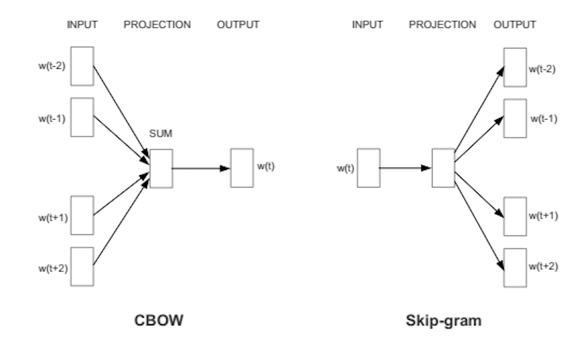
The above figure depicts the two training methods used in word2vec to learn word embeddings. On the left is the Continuous Bag of Words (CBOW) method, and on the right is Skip-Gram. At a high level, the CBOW and skip-gram model are opposites. The former learns to predict a word given that words context, the same way we did the example about the cat above. The latter learns to predict context given a word.

Both of these use some principles from convolutional neural nets, which are outside the scope of this article⁴. All you need is to think of these processes as black boxes that take vectors as input, and refine their result quality by comparing their output with our existing vectors.

Initially, all words are initialized as a random vector. Then we start scanning through all of the sentences in our training corpus. For each word, we pull out a number of that word’s neighbors. Then, using either method, we attempt to find word representations. We use the error between our predicted vectors and the randomly initialized ones in order to improve our model. We also occasionally swap a word’s representation with the output of our model.

By this process, word2vec eventually both finds a model which can predict word vectors given context (or vice-versa) as well as a set of word vectors that maximize the quality of that predictive model. This gives us $R(x)$, for all our words, which we can use in a number of ways to find embeddings for our documents. One of the simplest ways to do this is by simply averaging all of a document’s word vectors together.

$$ R(d_j) = \frac{\sum_{w_i \in W_j} R(w_i) )}{ |W_j| } $$

So now what?

Okay, so now that we have the fancy word vectors, we can do a lot of things with them. For example, imagine we wanted to find news articles related to Google. Well, we could find a large number of them by selecting documents whose vector representation is close to $R(\text{Google})$.

By using these representations, we can so improve the quality of our classifiers. Anywhere we used to use a BOW representation, we can replace that with a more efficient and more descriptive vector. Adding to the benefits, the length of the word2vec embeddings does not change based on the size of our vocabulary.

In Conclusion

I hope this helped give a background on word vectors, and at least brought you up to speed with this new method. Certainly, there is a lot more I could go into, and a lot of work is being done to apply this principle to solve a wide range of problems. But that will have to be the focus of a different post.